| |
| Volume 5, Number 1 | January/February 1999 |
Eight months ago I announced the conclusion of my effort to unify Biblical and secular chronologies back to the time of the Flood (roughly 3500 B.C.).[1] Since that time I have been embarked on a mission to unify sacred and secular chronologies in the period of time before the Flood. The present issue is the fourth in a series seeking this unification.
Once the missing thousand years in 1 Kings 6:1 is recognized and allowed for, no divergence between sacred and secular chronologies appears until the creation of Adam, roughly 5200 B.C.[2] At that point one encounters the "central conundrum" of Pre-Flood Biblical chronology, which is the apparent existence of mankind, according to secular scholarship, many thousands of years before the creation date of Adam determined from Biblical chronology.[3] One must somehow resolve this conundrum before sacred and secular chronologies can be unified.
I have enumerated nine conceptually possible solutions to this conundrum. I believe these nine exhaust the possibilities.[4]
The Biblical chronological data leading to the creation of Adam are false (i.e., fabricated).
The secular chronological data leading to a great antiquity for mankind are false (i.e., fabricated).
The Biblical history which teaches that Adam was the first man to be created is mythological or otherwise fabricated.
The modern secular teaching that mankind existed in remote antiquity is a hoax or fabrication.
We have misunderstood the Biblical history of the creation of Adam; the Bible does not really teach that Adam was the first man ever to be created.
The archaeologists have misunderstood the history of mankind; archaeology does not really show the existence of humans before Adam.
We have made some mistake in the computation of the Biblical date of the creation of Adam (i.e., the basic Biblical chronological data are valid, but they have been misunderstood).
The secular chronologists have made some mistake in their computation of the antiquity of man (i.e., the basic secular chronological data are valid, but they have been misunderstood).
The Biblical and secular evidences must both be accepted as legitimate; the truth lies in a proper synthesis of the two.
The eighth possibility leads directly to the question, "Radiocarbon dating—can you trust it?"[6] Last issue I introduced a set of sixty radiocarbon dates from the archaeological site of ancient Jericho to be used as a case study in answering this question. Detailed evaluation of these radiocarbon dates revealed that they harmonize with Biblical and secular historical expectations back to the time of the Flood. This showed that radiocarbon can be trusted to provide reliable absolute dates back to 3500 B.C. The only question remaining—the focus of the present issue—is whether radiocarbon dating is reliable prior to the Flood.
While radiocarbon dating is seen to be reliable at Jericho back to the time of the Flood, is it possible that something was different before the Flood? Is it possible the Flood itself changed something—such as the radioactive decay rate—so that the accuracy of radiocarbon dating is thrown off in the pre-Flood period?
I think it is the case that nobody has ever investigated this question as critically and as thoroughly as I have. It was to get to the bottom of the reliability of radiometric dating methods that I chose the particular Ph.D. program I did some two decades ago, and my decision to join the faculty of the Institute for Creation Research Graduate School following graduation was entirely motivated by my concern to plumb the depths of this question. The reliability of radiocarbon dating is of extreme importance to Biblical chronology and to our whole understanding of the past. To the one who wishes to accurately harmonize Biblical and secular accounts of earth history it is worth every ounce of effort and every bit of personal pain it may cost to get to the bottom of this question. I prosecuted this question very critically through every means available to me for over a decade. I entered this investigation with an extreme prejudice against the reliability of radiocarbon dating, and I emerged from it over a decade later with an assured and unqualified conviction that, yes, radiocarbon dating can be trusted in the pre-Flood period, back at least until 9000 B.C.
But, as usual, I do not want you to take my word for it simply because I claim considerable devotion to this question. I want, rather, to explain, as simply and clearly as I can, why it is I find "yes, radiocarbon dating is reliable in the pre-Flood period" to be the unavoidable truth. While I cannot take you through ten years worth of false starts and down a decade worth of blind alleys in the following few pages, I am hopeful that the following positive presentation of basic factual data will suffice to show this truth.
The single most important fact to grasp about radiocarbon dating in the period of interest to the present study (i.e., back to about 9000 B.C.) is that radiocarbon dates are calibrated using tree-rings over this entire range. This makes changes in the past behavior of radiocarbon—hypothetical changes in its decay rate, or alterations in the initial amount of radiocarbon in living things—irrelevant. Calibrated dates are immune to any such changes.
There is nothing tricky about how this happens, and nothing very complex about the idea of calibrating radiocarbon dates using tree-rings. Here are the basic concepts.
Radiocarbon—a radioactive form of the carbon atom—is produced in the atmosphere through the action of cosmic radiation on air molecules. Once produced, radiocarbon mixes with stable carbon atoms already in the atmosphere in the form of carbon dioxide. Because the atmosphere mixes thoroughly and rapidly (which is what wind and storms are all about) the ratio of radiocarbon to stable carbon is uniform all over the globe at any given time.[7]
Trees and other terrestrial plants get the carbon atoms they need to build their tissues from atmospheric carbon dioxide. As plants take in carbon dioxide from the atmosphere, they take in both radiocarbon and stable carbon atoms, in the ratio these are found in the atmosphere. Because this ratio is everywhere the same at the same time in the atmosphere, all of the terrestrial plants growing at the same time at every location over the entire globe have the same ratio of radiocarbon to stable carbon.[8] Animals get the carbon they need for building their tissues by eating plants (or by eating other animals which have gotten their carbon by eating plants). Thus, both the terrestrial plant and animal kingdoms contain the same ratio of radiocarbon to stable carbon atoms in their tissues while living at any point in time. This ratio may fluctuate from decade to decade, because the ratio of radiocarbon to stable carbon in the atmosphere may change with time. But at any given time the ratio will be the same globally for all terrestrial plants and animals then living.
When a plant dies, it ceases to take in carbon dioxide from the atmosphere. Radiocarbon atoms slowly disappear from its tissues because, being radioactive, they slowly decay away. Thus, the ratio of radiocarbon to stable carbon atoms in dead tissue slowly decreases. Because this decay process is a nuclear phenomenon, it is impervious to normal environmental factors such as temperature and humidity. Thus, the ratio of radiocarbon to stable carbon atoms will decrease in lockstep in all tissues of all terrestrial plants and animals which ceased to metabolize at a given point in time. It is this fact which is exploited by the radiocarbon calibration method of dating.
In the radiocarbon calibration method, tree-rings whose ages are precisely known through direct counting of growth rings back from the present time, are used to construct a table (or graph). One column of the table contains the calendar date when each tree-ring grew. Opposite this date, in another column, is recorded the experimentally measured ratio of radiocarbon to stable carbon found for that specific tree-ring today.
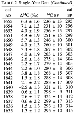
Figure 1 shows a small portion of an actual calibration table. Each line in this table represents one tree-ring. The column at left (first column) is the calendar age of the ring, obtained by counting rings back from the present. The column at right (fourth column) is just another way of expressing the tree-ring count. It gives calendar years before present (B.P.), with 0 B.P. defined as 1950 A.D. The second column tells what the radiocarbon ratio in the atmosphere was when each ring grew, relative to wood which grew near 1850 A.D. (before the industrial revolution began to add a great deal of stable carbon into the atmosphere). This is determined by direct measurement on each ring. The third column gives the measured conventional radiocarbon ages of the tree-rings. This is just a traditional way of expressing the (fractionation corrected) ratio of radiocarbon to stable carbon atoms in the tree-rings. Calibration tables like this one (though generally giving results for every ten or every twenty rings, rather than for each and every year) now exist based upon a series of nearly 12,000 consecutive tree-rings stretching backward in time from the present.[9]
 |
Suppose we would like to radiocarbon date a leather sandal found in ancient native American ruins in California. We do this today as follows. We first measure the ratio of radiocarbon to stable carbon atoms in the leather. (More accurately stated, we send the leather to a lab equipped to make such a measurement—along with three or four hundred dollars to pay to have this work done for us.)
Once we have this fundamental ratio, we go to the calibration table. We look in the table until we find a tree-ring sample having this same ratio. Since these two samples—the leather from the sandal and the wood from the tree-ring—have the same radiocarbon to stable carbon ratio today they are in lockstep at present.[10] This implies that they must both have ceased to metabolize (or died) at the same time, so they could begin their lockstep progression to the present time. We can, therefore, determine when the deer died, from which the leather for the sandal came, by looking at the adjacent column in the calibration table showing how many tree-rings ago that particular tree-ring was formed. This number will equal the number of years which have elapsed since the deer was killed by the native American, as long as each tree-ring in the calibration table corresponds to one calendar year.
Now we obviously must ask whether we can be confident each tree-ring in the calibration table does, in fact, correspond to one calendar year. And we will want to ask other probing questions about the tree-rings used to construct this calibration table, of course. But before we do let me emphasize that the whole burden of proof for the calendar reliability of radiocarbon dates has now shifted entirely away from the past behavior of the radiocarbon atom. Assumptions about the past decay rate of radiocarbon, or its initial concentration in the atmosphere, are irrelevant, as far as accuracy of the dates one obtains are concerned, when the calibration method is used. If the decay rate of radiocarbon was somehow altered by the Flood (and I know of no way to accomplish such a thing apart from explicit supernatural intervention, which the Biblical record of the Flood does not hint at) then this decay rate would have altered in all samples, including the tree-rings. In that case the ratio of radiocarbon to stable carbon would have remained in lockstep just the same, so the calibrated date would not be altered.
This is the important point. In the calibration method of radiocarbon dating—which all radiocarbon scientists now employ—the burden of proof for calendrical accuracy is shifted away from radiocarbon and onto the shoulders of dendrochronology, the science of counting tree-rings. Questions concerning the past behavior of radiocarbon itself—whether the Flood might have altered its radioactive decay rate, or whether the Flood might have caused a disequilibrium between present-day production and decay of radiocarbon, or any other such thing—do not impinge upon the accuracy of calibrated radiocarbon dates. In the quest to unify pre-Flood sacred and secular chronologies such questions are irrelevant.
Obviously, we must turn our attention away from the past behavior of the radiocarbon atom and focus it on the past behavior of tree-rings if we are to gain any real insight into the trustworthiness of pre-Flood calibrated radiocarbon dates. The critical question is not, "Can radiocarbon be trusted?" but rather, "Can dendrochronology be trusted?"
This was a difficult question to answer when the calibration method of dating first began to be developed. The only tree-rings extending far enough back in time to be of much use for calibration purposes at that time were from the remarkable bristlecone pine trees growing at high altitudes in the White Mountains of California.[11] These trees grow very slowly (Figure 2) and live to very great ages—some more than 4,000 years. Because of their resinous nature, and the cold, arid environment in which they grow, dead bristlecones can be preserved for thousands of years. By overlapping ring patterns in dead and living bristlecones, dendrochronologists had been able to construct a continuous series of bristlecone tree-rings extending from the present back 7100 rings into the past. This tree-ring series provided the basis of the earliest calibration table.
 |
But how was this bristlecone tree-ring series to be checked for calendrical accuracy? What if the dendrochronologists had matched the ring patterns incorrectly between two or more bristlecone specimens? One could certainly imagine an inadvertent duplication of a whole section of the series, artificially extending it thousands of years beyond its true range. And how could one be sure that these bristlecone pine trees only put on one growth ring each year?
To answer such concerns some sort of independent check on the bristlecone pine tree-ring chronology was needed. One desired to see a second, independent, calibration table, constructed using independently counted tree-rings. The calibration method could then be checked by seeing whether both calibration tables gave the same calibrated dates for all samples.
A small step in this direction was taken early on by comparing dendrochronologies from other types of trees, such as Douglas fir, to the bristlecone chronology. It was found that these agreed. But the ring series from these other trees were not nearly as long as the bristlecone pine series. This meant that only the most recent portion of the bristlecone chronology could be checked. Furthermore, all of the trees involved were from a single geographical region—the west coast of the United States. What was really needed was an independent, long dendrochronology from an entirely different part of the world. Fortunately, such a check was not long in coming.
Dendrochronologists were actively building long tree-ring chronologies not only in America, but also Europe. The European scientists found that they were able to construct a very long tree-ring chronology using oak trees. The younger portion of this chronology was pieced together from oak logs which had been used (and hence preserved) in the construction of various historic buildings. The chronology was then extended to more ancient times using older oak logs found preserved, for example, in ancient peat beds.
The European oak chronology was just what was needed to check the American bristlecone pine chronology. The two were obviously independent. Ring width patterns are determined by local environmental factors, such as temperature and rainfall. Since the specimens involved in these two chronologies grew on two separate continents, with an ocean between, there was no way the ring thickness pattern in one could act as any guide to the construction of the other. Furthermore, political boundaries assured that the scientists who worked on the oak chronology were different from, and independent of those involved in the bristlecone chronology.
Finally, the very different natures of the two types of trees involved—bristlecone and oak—was a significant advantage. Bristlecones are evergreens which grow very slowly, at high altitude, in a cold, arid environment, and live for thousands of years. None of these things is true of the oaks used in the European chronology. They are deciduous, grow relatively rapidly, at low altitudes, in relatively warm, moist environments, and live for only hundreds of years.
Did these two dendrochronologies yield calibration tables in harmony with one another? The answer is an unequivocal yes. Figure 3 illustrates a portion of what was found when these two dendrochronologies were compared through their respective radiocarbon to stable carbon ratios. More recently, Stuiver et al. have reported:[12]
[Radiocarbon] results determined in different laboratories for samples of the "same" dendroage usually yield offsets in the 0–20 [radiocarbon] year range. Values twice as large are occasionally encountered.That is, the largest offsets between labs over the entire series of nearly 12,000 consecutive tree-rings available today are forty years or less. The possibility of miscounted or misplaced thousands of rings in these dendrochronologies is immediately removed by these observations. It is clear that the dendrochronologists know how to assemble their tree-ring samples correctly.
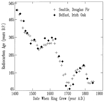 |
Furthermore, Figure 3 makes it clear that radiocarbon does, indeed, have a uniform distribution in the atmosphere, at least in the northern hemisphere. It shows that trees grown at the same time on separate continents have the same ratio of radiocarbon to stable carbon in their wood. This experimentally verifies the fundamental premise upon which the calibration method of radiocarbon dating is based.
The only question remaining at this point—and though one may appear a severe skeptic even to ask it, let us leave no stone unturned—is whether it might just be possible that both of these dendrochronologies have incorporated multiple ring growth per year. Suppose, for example, that the trees used in these long dendrochronologies, both in America and in Europe, have a propensity for adding, not one growth ring each year, but two growth rings per year on average. If these rings were all treated as annual growth rings, then the dendrochronologies would appear to show a factor of two too many calendar years.
We know that calibrated radiocarbon dates are accurate back to the time of the Flood, and this means that the tree-ring count that these dates are based upon must also be accurate from the present back to that time. Thus, we know the trees used in constructing these long dendrochronologies, on two separate continents, were only growing one ring per year from the Flood down to the present time. But is it possible that something was different before the Flood, so that pre-Flood trees routinely grew two or more rings each year? Is it possible that multiple ring growth per year prior to the Flood is the explanation of the pre-Adamic calibrated radiocarbon dates from human remains at Jericho?
It is possible to test the hypothesis of multiple ring growth per year before the Flood using the calibration table itself. The idea here is fairly simple. To illustrate it, imagine for a moment that there exists an aged magician who has the power to cause trees to grow brilliantly blue growth rings. In the years when he does not exercise this power all the trees in his world grow normal-colored growth rings for that year. But in the years when he does exercise his power, all the trees grow brilliant blue rings during that year. As a result, when you cut a tree down in the magician's world and examine the growth rings you observe a pattern of brilliant blue rings interspersed among normal rings.
Now what motivates this magician to exercise his power is not known, but what is well known is that whenever he starts to cause the trees to grow blue rings he keeps it up for exactly ten years in a row before stopping again.
Given this odd behavior it is a simple thing to detect multiple ring growth in the trees of the magician's world. If you cut a tree down and find a group of fifteen sequential blue rings, then you know that tree was not adding one growth ring per year. This immediately follows because we know the magician always exercises his power in ten year blocks. The extra five rings are evidence that the tree put on more than one ring per year during some of the years of that ten year span. If, on the other hand, you find that blue rings appear only in groups of ten, then you know that the trees have only been growing one ring per year.
In this analogy the magician represents the sun. The sun occasionally, for unknown reasons, goes into a relatively quiescent mode of operation.[13] During such episodes few sunspots are seen on the surface of the sun, and the solar wind is reduced. This lets more cosmic radiation into the upper atmosphere of the earth, which allows more radiocarbon atoms to be produced in the atmosphere. Eventually the sun returns to normal operation and radiocarbon returns to normal levels in the atmosphere once again. But the result is that the ratio of radiocarbon to stable carbon atoms in the atmosphere goes through occasional small "peaks". Since the trees are simply "recording" whatever ratio of radiocarbon to stable carbon is in the atmosphere at the time they put on each growth ring, the rings themselves are permanently "dyed" with these higher than usual radiocarbon levels. These are the tell-tale "blue" rings.
Now, contrary to the magician of my analogy, our sun exhibits not one, but two quiescent modes. One mode lasts roughly 51 years on average, and the other about 96 years on average. We could expand our analogy and imagine that the magician paints growth rings blue for ten years at a time, while at other times he paints them red for twenty years at a time. This adds complexity to the analogy, however, which is why I have left it out above. The basic idea, I think, is nonetheless clear.
Examples of both quiescent modes are visible in Figure 3. These appear as valleys in the figure, rather than peaks, since radiocarbon "age" decreases whenever the ratio of radiocarbon to stable carbon increases. A valley resulting from the 51 year sort of solar quiescence dips to a minimum near A.D. 1700, and another, of the 96 year variety, reaches its minimum just after A.D. 1500. The valley near 1700 is known as the "Maunder minimum" and the one near 1500 is known as the "Sporer minimum".
Now let us get down to quantitative business with this. Our immediate concern is to decide whether the calibrated radiocarbon dates from Jericho which appear to predate the creation of Adam are trustworthy. We are asking whether their apparently excessive age might be due to multiple ring growth per year prior to the Flood in the dendrochronologies upon which their ages are based.
How many rings per year would the trees need to have grown pre-Flood on average to bring the oldest radiocarbon dates at Jericho down in age so that they are equal to the creation date of Adam?
Figure 4, reproduced here from last issue, shows that the calibrated radiocarbon dates in question go back at least to a putative 8500 B.C. Meanwhile, we know that the Flood happened approximately 3500 B.C. Thus, 5000 growth rings separate the Flood from the oldest human remains dated by the calibration method at Jericho.
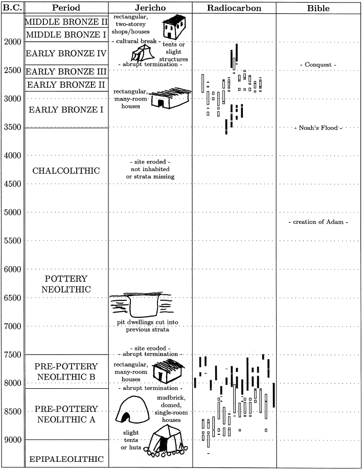 |
We would like to try to compress these 5000 growth rings into just the span of time from the Flood back to Adam's creation. That span of time, we know from Biblical chronology (see Figure 4), is 1700 years.
To compress 5000 growth rings into 1700 years, the trees must have been growing (5000/1700=) 2.9 rings per year on average in the pre-Flood period.
If the trees were growing 2.9 rings per year in the pre-Flood period, then the sun-induced "peaks" in the ratio of radiocarbon to stable carbon measured in the rings (the "blue" and "red" rings) should occupy approximately (2.9×51=) 148 growth rings and (2.9×96=) 279 growth rings on average respectively, instead of their normal average of 51 and 96 growth rings. Do they?
Figure 5 shows that, in point of fact, they don't.[14] Each circle in the figure represents one "peak". I found seven peaks before the Flood and nine peaks after the Flood.
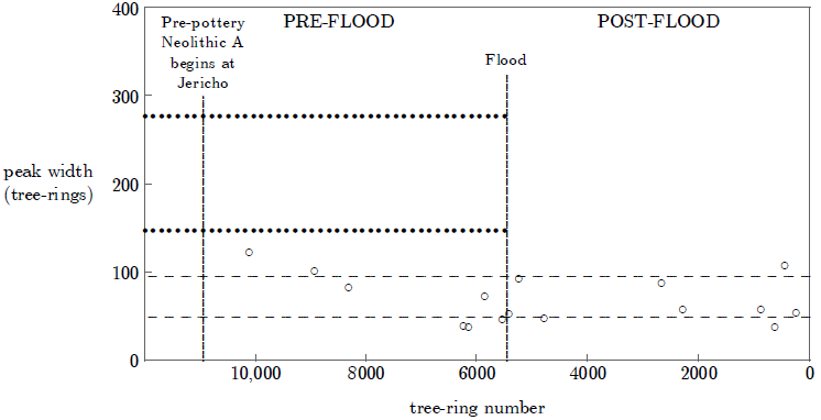 |
Three of the nine post-Flood peaks are of the 96-year type. The average of their widths is 96 years (which is where the 96 year figure comes from). This average is plotted as the upper horizontal dashed line in the figure.
The average of the remaining six post-Flood peaks is 51 years. This is plotted as the lower dashed line.
The dotted horizontal lines show 2.9 times the post-Flood peak widths. The upper dotted line corresponds to the upper dashed line, and the lower dotted line corresponds to the lower dashed line.
If pre-Flood trees were growing 2.9 rings per year on average, then the pre-Flood peaks should all cluster around the upper and lower dotted lines, just as the post-Flood peaks cluster around the dashed lines. But they don't. The pre-Flood peaks continue to cluster around the dashed lines. Apparently, there was no significant difference in the growth characteristics of the trees pre-Flood and post-Flood. The hypothesis that trees in the pre-Flood period were growing multiple rings per year is falsified.
This means that the apparently excessive ages of the earliest calibrated radiocarbon dates from Jericho can not be explained away as due to multiple tree-ring growth per year prior to the Flood. Five thousand truly annual growth rings do, indeed, separate early human remains at Jericho from the Flood. And this means that some 3300 truly annual growth rings separate these early human remains from the creation of Adam. The evidence for the apparent existence of mankind thousands of years before the creation date of Adam is unambiguously affirmed at Jericho.
Now I hope that you will agree with me that the "central conundrum" of pre-Flood Biblical chronology is properly named. Here is a conundrum indeed.
The Bible, we have seen, seems to teach that Adam was the first man ever to have existed.[15] When coupled with the doctrine of Biblical inerrancy this leads immediately to what I will call Grand Fact 1.
Grand Fact 1 Adam was the first human ever to have existed.
Meanwhile, the data from the ground at Jericho lead immediately to Grand Fact 2.
Grand Fact 2 Human remains and artifacts exist which greatly predate Adam.
These two Grand Facts seem logically incompatible. One's immediate reaction is to seek to reject one or the other of them. But try as we might, no rational way of rejecting either of them appears.
I have been reading and studying in the field of ultimate origins for at least a quarter of a century now. During this time I have seen a broad range of ideas about the origins of mankind and the meaning of Genesis. I have observed that these ideas, almost without exception, exercise themselves in an attempt to deny one or the other of these Grand Facts. Most, these days, seek to deny Grand Fact 1. But, as far as I have been able to see, none of these ideas, whether secular or theological at root, has ever actually succeeded in demonstrating any rational way of denying either Grand Fact 1 or Grand Fact 2.
I have never yet found anybody who has ever been able to show any legitimate way of setting either of these Grand Facts aside, and I can conceive of no way of doing so myself. This leads me to conclude that apparently, difficult though this may seem, truth is to be had, not by a rejection of one or the other of these Grand Facts, but by embracing both of them together.
This brings us to our ninth and final possible solution.
The Biblical and secular evidences must both be accepted as legitimate; the truth lies in a proper synthesis of the two.
Can a workable synthesis of the Biblical and secular evidences for the antiquity of mankind be found? I'll be taking a look at this question next issue, Lord willing. ◇
The Biblical Chronologist is a bimonthly subscription newsletter about Biblical chronology. It is written and edited by Gerald E. Aardsma, a Ph.D. scientist (nuclear physics) with special background in radioisotopic dating methods such as radiocarbon. The Biblical Chronologist has a threefold purpose: to encourage, enrich, and strengthen the faith of conservative Christians through instruction in Biblical chronology, to foster informed, up-to-date, scholarly research in this vital field within the conservative Christian community, and to communicate current developments and discoveries in Biblical chronology in an easily understood manner. An introductory packet containing three sample issues and a subscription order form is available for $9.95 US regardless of destination address. Send check or money order in US funds and request the "Intro Pack." The Biblical Chronologist (ISSN 1081-762X) is published six times a year by Aardsma Research & Publishing, 412 N Mulberry, Loda, IL 60948-9651. Copyright © 1999 by Aardsma Research & Publishing. Photocopying or reproduction strictly prohibited without written permission from the publisher.
|
^ Gerald E. Aardsma, "Biblical Chronology 101," The Biblical Chronologist 4.3 (May/June 1998): 6–10.
^ Gerald E. Aardsma, A New Approach to the Chronology of Biblical History from Abraham to Samuel, 2nd ed. (Loda IL: Aardsma Research and Publishing, 1993); Gerald E. Aardsma, "Toward Unification of Pre-Flood Chronology," The Biblical Chronologist 4.4 (July/August 1998): 1–10.
^ Gerald E. Aardsma, "Toward Unification of Pre-Flood Chronology," The Biblical Chronologist 4.4 (July/August 1998): 10.
^ Gerald E. Aardsma, "Toward Unification of Pre-Flood Chronology: Part II," The Biblical Chronologist 4.5 (September/October 1998): 1–10.
^ Gerald E. Aardsma, "Toward Unification of Pre-Flood Chronology: Part II," The Biblical Chronologist 4.5 (September/October 1998): 1–10.
^ Gerald E. Aardsma, "Toward Unification of Pre-Flood Chronology: Part III," The Biblical Chronologist 4.6 (September/October 1998): 1–16.
^ Slight deviations from complete uniformity can be demonstrated, especially between the northern and southern hemispheres, whose atmospheres mix together relatively slowly. But these departures from complete uniformity are too small to be of any practical importance to the present discussion.
^ Biological fractionation can bring about small alterations in the ratio of radiocarbon to stable carbon in plant tissues from one species to another. This effect is too small to be of any practical significance in the present context, and it can be experimentally corrected for when the ratio of radiocarbon to stable carbon is measured in a sample in any event.
^ See, for example: Minze Stuiver, Paula J. Reimer, and Thomas F. Braziunas, "High-precision Radiocarbon Age Calibration for Terrestrial and Marine Samples," Radiocarbon 40.3 (1998): 1127–1151.
^ I have skipped over the possibility of two or more tree-rings, which grew at different times, having the same ratio. This can happen (and frequently does) because the ratio of radiocarbon to stable carbon in the atmosphere fluctuates up and down with time. This effect can introduce more than one possible date range, usually within a few hundred years of each other, for a given sample. However, this effect is of no practical significance in the present context, which is seeking to show only that calibrated radiocarbon dates cannot possibly all be out by the thousands of years necessary to solve the central conundrum.
^ C. W. Ferguson, "Bristlecone Pine: Science and Esthetics," Science 159 (23 February 1968): 839–846.
^ Minze Stuiver, Paula J. Reimer, Edouard Bard, J. Warren Beck, G. S. Burr, Konrad A. Hughen, Bernd Kromer, Gerry McCormac, Johannes Van Der Plicht, and Marco Spurk, "INTCAL98 Radiocarbon Age Calibration, 24,000–0 cal BP," Radiocarbon 40.3 (1998): 1041–1083.
^ M. Stuiver and P. D. Quay, "Changes in Atmospheric Carbon-14 Attributed to a Variable Sun," Science 207 (1980): 11–19.
^ I used the Δ14C data from the INTCAL98 calibration curve for this figure. The data were downloaded over the Internet from the Quaternary Isotope Laboratory in Seattle, Washington (http://depts.washington.edu/qil/). I selected all peaks in the time span of interest which were large and well defined. Sixteen peaks total were found. To furnish an objective measure of the width of these peaks I performed a least squares fit of a Gaussian plus linear background to each peak.
^ Gerald E. Aardsma, "Toward Unification of Pre-Flood Chronology: Part II," The Biblical Chronologist 4.5 (September/October 1998): 1–10.